
Inside Java
News and views from members of the Java team at Oracle
News and views from members of the Java team at Oracle
The work presented here is performed as part of the joint research project between Oracle, Uppsala University and KTH. Follow the blog series here at inside.java to read more about the JVM research performed at the Oracle Development office in Stockholm.
My name is Emmy Yin and I am currently finishing up my engineering degree within theoretical computer science at KTH. During the spring 2023, I got the opportunity to write my Master's thesis at Oracle. My thesis revolved around Ideal Graph Visualizer (IGV) and the purpose was to explore graph layout algorithms for visualizing dynamic graphs.
Writing my thesis at Oracle has been a rewarding experience. I would like to thank the people at Oracle Stockholm and Zürich for it. I have truly learnt a lot during my project. A special thanks to Roberto Castañeda Lozano and Tobias Holenstein for supervising me throughout the thesis!
IGV is a graph visualization tool that is part of OpenJDK. It was developed to help engineers understand, debug and enhance OpenJDK's main just-in-time (JIT) compiler C2. The JVM represents a program under compilation as a dynamic Intermediate Representation (IR) graph that changes as the program is being compiled. IGV is a tool for visualizing the IR graphs. More information can be found here. To visualize the graphs, IGV uses a static graph layout algorithm. This means that only the current state of the graph that is to be visualized is considered, without accounting for any changes that have occurred to obtain the graph. The benefit is that the algorithm can focus on drawing a layout of high quality, that is easily read and understood. However, the drawback is that a small change to the graph can cause a major relayout, making it difficult to see what changes actually occurred.
Let's illustrate this with an example. A graph G is visualized like this: 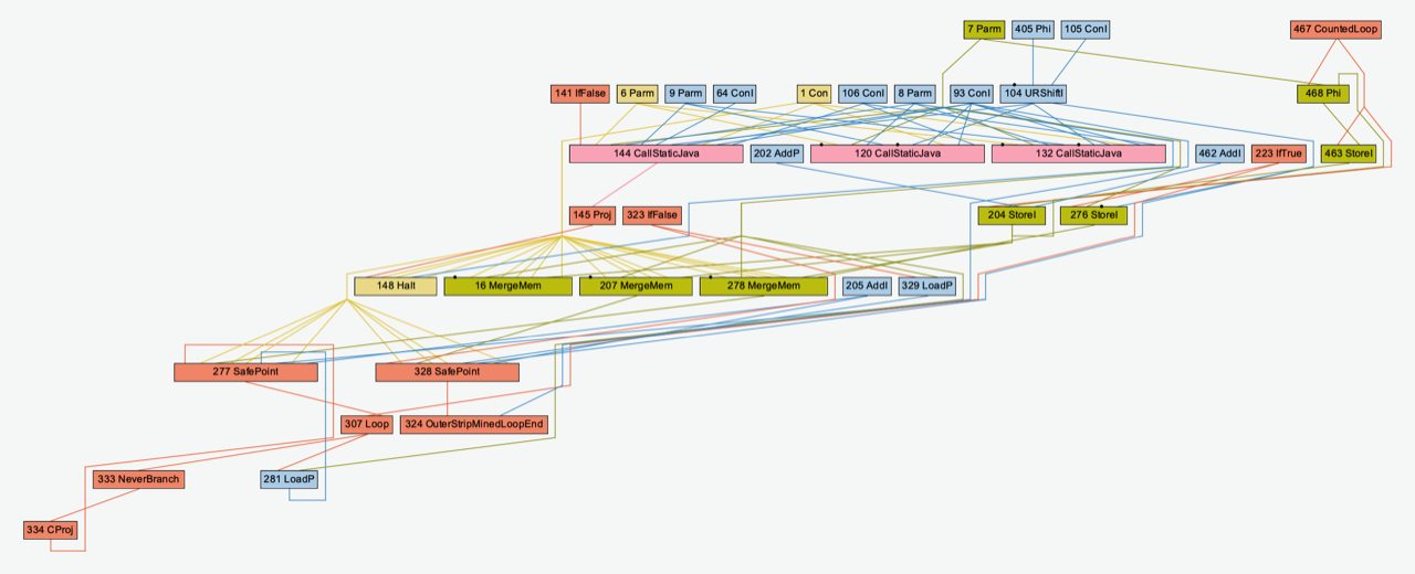
The nodes are grouped into layers, so that there is a flow from the topmost layer downwards. In this layout, we have a total of nine layers, with nodes 7, 405, 105 and 467 on the topmost layer, and node 334 on the last layer.
One node is added to the graph along with one edge, creating a new graph G'. The static algorithm draws the layout of G' as such, where the added node is circled in red: 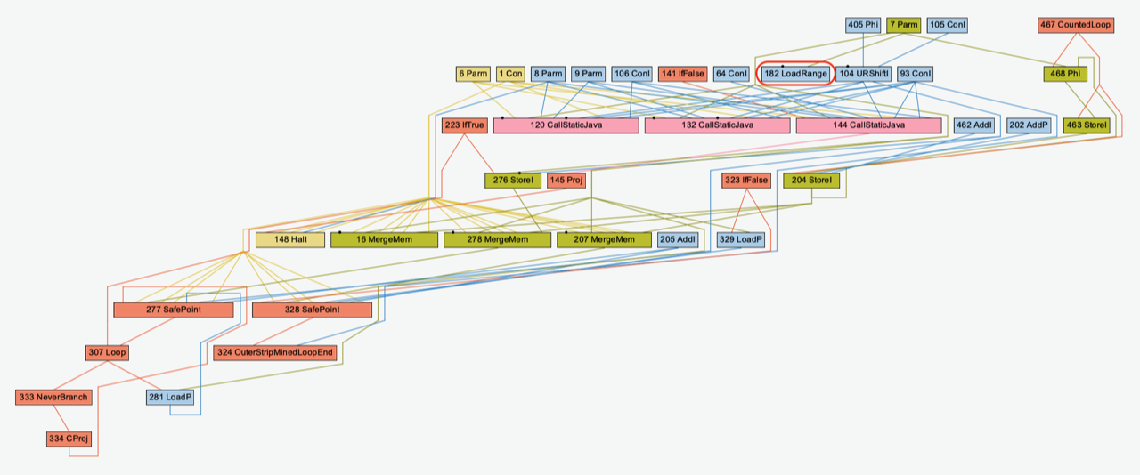
At a first glance, the layouts look very similar. But when analyzing them more closely, it is noticeable that the order of the nodes in each layer has changed. The reason for the reordering of the nodes is to minimize edge crossings, making the layout slightly easier to read. The reordering can however be misleading and confusing for the viewer.
In my thesis, I implemented a dynamic layout algorithm as an alternative to the static one. The idea behind the algorithm is to apply update actions on the previous layout incrementally to obtain the new layout. The steps of the algorithm are:
Identify all changes between the previous graph state and the new.
Divide the changes into a sequence of update actions. Each action is one of the following:
Increase node size
Remove node
Add node
Remove edge
Add short edge (edge between nodes on adjacent layers)
Add long edge (edge that spans multiple layers)
Add edge between nodes on the same layer
Apply the actions in the following order:
Resize nodes
Remove nodes and edges
Add nodes
Add edges
Visualize resulting layout
The relative positions of the nodes that appear in both the previous and the new layout are therefore preserved. Continuing on the above example, the layout drawn by the dynamic algorithm for G' is shown below. Again, the added node is circled in red. 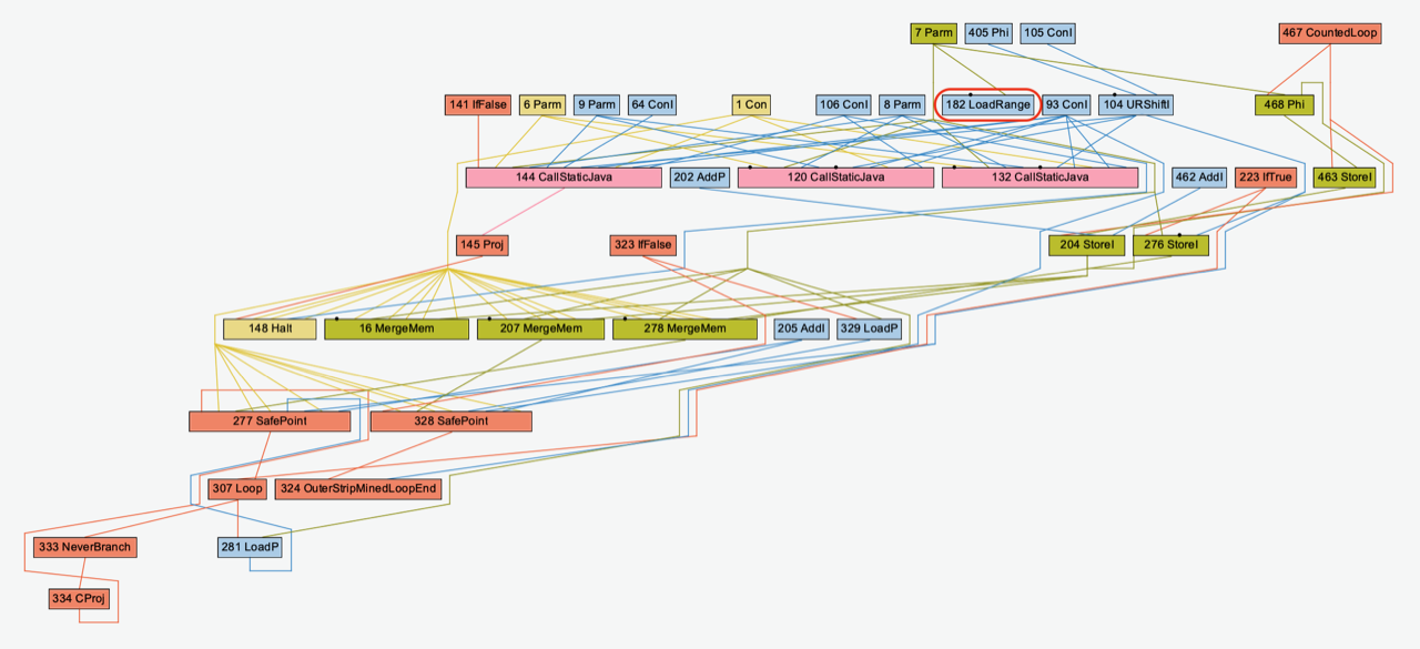
It is clear that the order of the nodes from the layout of graph G has been preserved, making it easier to identify the added node in G'.
I ran both algorithms on a large set of graphs to evaluate and compare them. The results indicated that the dynamic layout algorithm moves the nodes around less, leading to layouts that are more dynamically stable. The results are strong for small graphs with few changes. However, as the graphs grew in size, or the changes were too large, the stability decreased. Regarding the layout quality, it seems that the dynamic algorithm causes more edge crossings, reversed edges, edges that are more bent, and overall longer edges. This means the layouts are more cluttered and harder to read, compared to the layouts drawn by the static algorithm.
The dynamic algorithm might be a better choice when the expected changes are small or the viewer prioritizes dynamic stability, whereas the static algorithm is useful when it is important that the layout quality is high. There is a trade-off between layout quality and dynamic stability, which could be interesting to further explore.